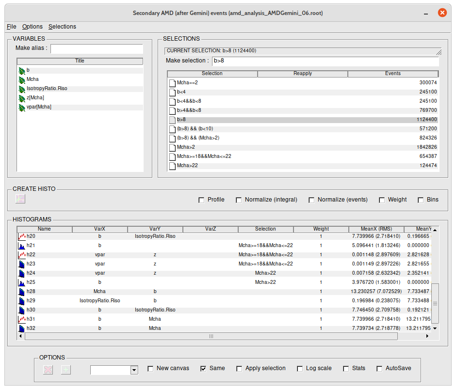
Figure 1: The kvtreeanalyzer GUI
kvtreeanalyzer is a graphical user interface (GUI) for analysis of data in TTrees and histograms. It can be used as an alternative to the standard ROOT TBrowser and TTreeBrowser GUIs. The main interest is that TTree analyses (including all generated histograms, selections, and TTree aliases) can be saved to file and continued or consulted at a later time, or even applied to data in another TTree (’automatic’ analysis). In ’autosave’ mode, displayed histograms can automatically be saved as image files in the user’s chosen directory. It uses a KVCanvas to display histograms, thus allowing easier manipulation of data through dynamic zoom, pan & scan, etc.
To open the kvtreeanalyzer GUI from the command prompt, either type
$ kvtreeanalyzer
in order to choose the file to analyze from the GUI, or, if you want to open directly a ROOT file with the GUI,
$ kvtreeanalyzer myfile.root
The first TTree found in the file will be connected for analysis.
New analysis
open a ROOT file containing a TTree and/or histograms to start a new analysis
Open analysis
open a ROOT file containing a previously-saved analysis session and reconnect the file containing the TTree
Add Friend...
open a second file and use the TTree in it as a “friend” (see ROOT documentation about Adding Friends to Trees)
Save analysis
save current analysis. Default file name is Analysis_toto.root where toto.root is the name of the file being analysed. If analysis was previously saved with a different filename (using ’Save as...’), the same filename will be used;
Save as...
save current analysis in a new file with user-specified name;
Close
close the currently analysed file
Apply analysis...
apply current analysis to a new TTree (see Automatic Analysisł::bel sec:Automatic-Analysis)
PROOF
activate (or deactivate) use of PROOFLite (on a multicore machine) to run analyses in parallel
Combine...
submenus are active when two or more selections are selected, allowing to generate a new selection which is either the logical AND or OR of the existing selections;
Update
if the analysed TTree has been updated since the last session, this will reapply all existing selections to the new data;
Delete
delete the selected selection(s)
Generate...Constant X-sections
generate selections with a given variable, with each selection corresponding to constant cross-section (same number of events). Opens a dialogue asking for the name of the variable to use, the total cross-section (can be 1) and the cross-section of each selection (can be < 1 if total cross-section is 1, i.e. allows to define the fraction of events in each selection).
In this panel is shown a list of all variables (leaves) and aliases of the currently analysed TTree, along with any aliases defined by the user with ’Make alias’ł::bel subsec:’Make-alias’. Any arrays appear with the (static or dynamic) dimension enclosed in ’[]’ after the name. Double-clicking on a variable in the list will cause the (1D) distribution of the variable to be drawn.
Allows to create a new alias expression which will be added to the list of variables. If the analysis is saved (see ’File’ menuł::bel subsec:’File’-menu) the new alias will be saved for future use. Enter any valid expression (any mathematical combination of leaves and existing aliases, TMath functions, or one of the Abbreviationsł::bel subsec:Abbreviations) and hit <ENTER>. Note that a single left-click on a variable in the list will copy its name into the ’Make alias’ box to avoid typing it.
The following abbreviations can be used in aliases and selection expressions:
TMath::DegToRad()
TMath::RadToDeg()
This panel allows to generate, apply and manage event selections. The currently active selection (if any) is displayed at the top of the panel. In order to apply a selection (it will be used for all histograms which are subsequently generated), double-click on it in the list. To deactivate the current selection (so that there is no active selection), double-click on the current selection in the list.
Selections can be created in several ways:
Write a valid logical expression (any mathematical combination of leaves and existing aliases, TMath functions, or any of the defined Abbreviationsł::bel subsec:Abbreviations) in the box and hit <ENTER>. Note that a single left-click on an existing selection in the list will copy it into the ’Make selection’ box to avoid typing it. The new selection will appear in the list along with the number of corresponding events.
Note1:
If a selection was already active, the new selection will be a combination (logical AND) of the existing selection and the new condition you entered.
Any existing selections can be combined either exclusively (AND) or inclusively (OR). Select the required selections in the list (left-click on the first, <CTRL>-left-click on the following) and use the ’Selections>Combine’ submenu (see ’Selections’ menuł::bel subsec:’Selections’-menu).
Graphical cuts (TCutG) can be used to generate selections from 2D histograms. Draw a closed contour in a 2D histogram, then change the name of the contour via its context menu. Double-click on the same 2D histogram in the HISTOGRAMS listł::bel sec:HISTOGRAMS-list, and the corresponding selection will be generated with the name of the contour in the selection list. The contour itself is added to the HISTOGRAMS listł::bel sec:HISTOGRAMS-list so that it will be saved with the analysis.
This list displays all histograms generated by the analysis, including any histograms found in the TTree file. Histograms can be displayed by double-clicking. Histograms can be deleted by selecting them (use <CTRL>-left-click or <SHIFT>-left-click for multiple selections) and clicking the DELETE button in the OPTIONS panelł::bel subsec:Options.
For each histogram, the variables/expressions used on x, y, and z axes, any selection and weighting, as well as the mean and standard deviation of the x and y expressions are displayed.
Double click on a leaf or alias in the VARIABLES panelł::bel sec:VARIABLES-panel. The new histogram (generated according to the selected Histogram creation optionsł::bel subsec:histogram-creation-options) will be added to the HISTOGRAMS listł::bel sec:HISTOGRAMS-list and will be displayed according to the currently selected option in the OPTIONS panelł::bel subsec:Options.
Note:
If a 1D histogram for the same leaf or alias for the current selection of events already exists, no new histogram will be generated: the existing histogram will be displayed. If no histogram exists for the current selection, it will be generated (no need for option ’Apply selection’ in this case, see OPTIONS panelł::bel subsec:Options).
Select two leaves or aliases in the VARIABLES panelł::bel sec:VARIABLES-panel (left-click on the first, <Ctrl>-left-click on the second). Their names will appear next to the familiar TTreeBrowser ’Draw’ button in the ’CREATE HISTO’ panel, separated by a semi-colon. The order of selection of variables is respected: if you want to plot toto (on the y-axis) as a function of tata (on the x-axis), click toto first and then tata: this will display toto:tata.
Click the ’Draw’ button to generate the histogram. The new histogram (generated according to the selected Histogram creation optionsł::bel subsec:histogram-creation-options) will be added to the HISTOGRAMS listł::bel sec:HISTOGRAMS-list and will be displayed according to the currently selected option in the OPTIONS panelł::bel subsec:Options.
Note1:
If a 2D histogram for the same combination of variables for the current selection of events already exists, no new histogram will be generated: the existing histogram will be displayed. If no histogram exists for the current selection, it will be generated (no need for option ’Apply selection’ in this case, see OPTIONS panelł::bel subsec:Options).
Proceed as for Generate a 2D histogramł::bel subsec:Generate-a-2D after having selected option ’Profile’ (see Histogram creation optionsł::bel subsec:histogram-creation-options).
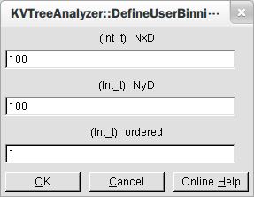
Select three leaves or aliases in the list (left-click on the first, <CTRL>-left-click on the second and third). Click the ’Draw’ button to generate the corresponding Dalitz plot (see KVDalitzPlot). If the 3 variables are size-ordered (i.e. x1 > x2 > x3 for all events) only one sixth of the Dalitz triangle will be covered: in this case, select option ’Bins’ (see Histogram creation optionsł::bel subsec:histogram-creation-options) and set the value of ’ordered’ in the dialogue box to ’1’ (see Fig.2).
Options which control creation of histograms:
Profile
select to generate a profile histogram from two variables selected in the list;
Normalize (integral)
choose this option to generate a normalized 1D distribution of a variable, by double-clicking on it in the VARIABLES panelł::bel sec:VARIABLES-panel. The normalization is such that the integral of the distribution is equal to 1;
Normalize (events)
choose this option to generate a normalized 1D distribution of a variable, by double-clicking on it in the VARIABLES panelł::bel sec:VARIABLES-panel. The normalization is with respect to the number of events corresponding to the current selection (useful when plotting e.g. array variables which can have several values for each event);
Weight
allows to define a binning weight for generating histograms. In the dialogue box which opens when ’Draw’ is clicked, enter an expression (any mathematical combination of leaves and aliases, TMath functions, Abbreviationsł::bel subsec:Abbreviations) which will be evaluated as a weight for each entry in the generated histogram. Logical expressions (which evaluate to 0 or some other value) can be used to select data to be included in the histogram - this is particularly useful when dealing with array variables;
Bins
allows to specify the number of bins and the limits of each axis for either 1D or 2D histograms, in the dialogue box which opens when ’Draw’ is clicked (see User-binning dialogue boxł::bel fig:User-binning-dalitz).
Several options for displaying histograms:
New canvas
display each histogram in a new canvas;
Same
superimpose next histogram on existing plot. For 1D histograms and profile spectra, each new addition will have a different colour, a TLegend will be automatically added to the canvas starting with the second plot and updated with further additions, and if the y-axis is insufficient to display the most recent histogram, it will be adjusted;
Apply selection
choose this option to generate a new histogram from an existing histogram by applying the event selection which is currently active (see SELECTIONS panelł::bel sec:SELECTIONS-panel). Double-click on the existing histogram to regenerate;
Log scale
display histograms with a logarithmic y-axis (1D, profile) or z-axis (2D, Dalitz plots);
Stats
option to display or not the histogram statistics box
AutoSave
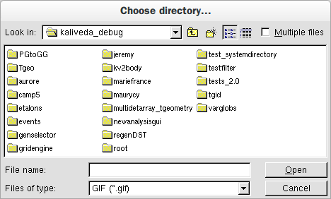
When ’AutoSave’ mode is active, every time a histogram is displayed the active canvas will be saved in a file with the format chosen by the user. When ’AutoSave’ is checked, the AutoSave directory and format choice dialogue boxł::bel fig:AutoSave-directory-and opens for the user to select the directory where files should be saved, and the format can be selected from the drop-down list: *.ps, *.eps, *.pdf, *.svg, *.tex, *.gif, *.root, *.xml, *.png, *.xpm, *.jpg, *.tiff, *.xcf.
Each time a histogram is double-clicked in the HISTOGRAMS listł::bel sec:HISTOGRAMS-list, it will be saved in the chosen directory with the required format, the filename is built from the histogram title (i.e. contains the plotted expressions and any applied selection), like this:
/autosave/directory/VAR1:VAR2_{SELECTION}.format
Automatic analysis allows to apply an existing analysis (set of selections and generated histograms) to new data stored in a TTree with the same leaf/alias list. Simply select ’Apply analysis...’ in the ’File’ menuł::bel subsec:’File’-menu and select a ROOT file containing the new data. A new kvtreeanalyzer GUI window will open containing the generated analysis.