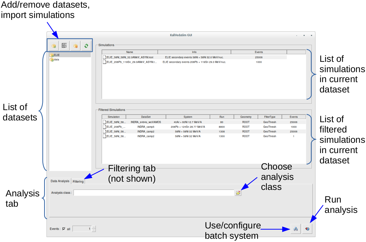
Figure 1: Overview of KVSimDirGUI
kaliveda-sim is a graphical interface which allows to manage simulated and filtered simulated data. It can be used to filter existing simulations with any known detector set-up, and to analyse both ’raw’ and filtered simulations. In fact it can handle any data which is stored in a branch in a TTree containing objects of a class derived from KVEvent. Different datasets can be managed, each one corresponding to a different disk directory containing data in ROOT trees. ROOT files in the dataset directories are automatically scanned to find TTrees with a branch containing objects either of a KVEvent-derived class or of a KVReconstructedEvent-derived class. The former files will be considered as simulated data, and the latter as filtered simulated data.
To launch the application from the command line, type
$ kaliveda-sim
The graphical user interface (see Fig.1) opens.
A dataset is a directory containing ROOT files with simulated and/or filtered simulated data contained in TTrees.
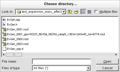
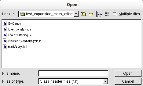
Click on the ’Add dataset’ button (see Fig.1). A file dialogue opens (Fig.2): navigate into the directory containing your simulation files and click the ’Open’ button.
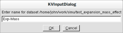
Next enter a name for your dataset in the dialogue box (Fig.3) and click the ’OK’ button.
The new dataset appears in the list of datasets, any existing simulated and/or filtered data in the directory are displayed in the respective lists.
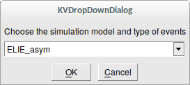
To add a new simulation to a dataset, select the dataset in question and press the ’Import simulation’ button (see Fig. 1). After selecting the file you want to import, a dialog box will open asking you to select the kind of simulation data (see Fig. 4). For each model there are two types of event: ’primary’ events corresponding to results of collisions before secondary decay (model name with no suffix) and ’asymptotic’ events after full secondary decay and propagation towards the detectors (model name with ’_asym’ suffix).
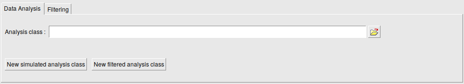
Clicking on one of the two buttons in the ’Analysis’ tab will generate an example analysis class for either simulated (non-filtered) or filtered data (N.B.: you have to use the right type of class for the data you want to analyse). You will be asked to give a name for the class. You can then open the generated ’.h’ and ’.cpp’ files in your favourite text editor in order to modify the class according to your needs.
In the ’Analysis’ tab, click on the analysis class selection button (see Fig.1). In the file dialogue box (Fig.6) navigate to the directory containing your analysis class files and select the appropriate header (’.h’) file. Remember that simulated (non-filtered) data should be analysed with a class generated by clicking the ’New simulated analysis class’ button, and filtered data with a class generated by clicking the ’New filtered analysis class’ button.
Adjust the number of events you want to analyse, or check ’All’ to analyse all events. Select one or more simulated or filtered data files in the corresponding list and click on the ’Run analysis’ button.
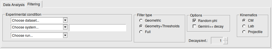
In the ’Filtering’ tab (Fig.7), select the dataset and collision system which define the experimental conditions for which you want to filter your simulation. The dataset defines the detector geometry with which to filter the data. The system defines the kinematics for the required boost to the lab (detector) frame in case your simulated data is in the centre of mass frame. Optionally, you can choose a specific run number; if not, the first run corresponding to the chosen system will be used.
If the collision you are simulating is not defined for your chosen dataset, you can enter an ad hoc system in the box next to the ’Choose system...’ list: the format to use is e.g. ’129Xe+119Sn@50.0MeV/A’ (if you hover over the box with the mouse, a tooltip will appear with this information).
Choose the filter type you want (see KVMultiDetArray::DetectEvent for more details):
Geometric - particles are considered detected if they hit at least one detector in the array;
Geometry+Thresholds - (recommended) charged particles must have sufficient energy to escape the experimental target and overcome realistic identification thresholds in order to be detected. Moreover, particles which stop in the same detector are rejected as unidentified, while a pseudo-coherency analysis of the particles in each group is used to decide whether they could be identified experimentally.
Full - (experimental) Full simulation of array response, inverted calibrations are used to generate pseudo-experimental raw data, which is then identified and calibrated using exactly the same experimental procedures. This is only possible for datasets which were entirely calibrated using KaliVeda.
Choose any options to use:
Random phi - (default) each simulated event will be given a random azimuthal rotation around the beam (z) axis before detection
Gemini++ decay - if your version of KaliVeda was compiled with Gemini++ support, this option will be available. The nuclei of each simulated event will be subjected to statistical decay using Gemini++ before detection. You can choose to perform more than one “afterburn” per simulated event by increasing the value of ’Decays/evt.’. If this is greater than one, each simulated event will be ’decayed’ and ’detected’ N times.
Specify the kinematics of the simulated data:
CM - the simulated data was generated in the centre of mass frame. Before detection simulation, the centre of mass velocity corresponding to the specified colliding system will be used to transform particle momenta into the laboratory frame
Lab - the simulated data was generated in the laboratory frame, no transformation is required before filtering
Projectile - the simulated data was generated in the projectile frame. Before detection simulation, the projectile velocity corresponding to the specified colliding system will be used to transform particle momenta into the laboratory frame
Select a simulated data file in the list and click on the ’Run filter’ button. The new file of reconstructed filtered data (pseudo-experimental data) will be written in the same directory as the simulated data file: the new file will appear in the ’Filtered simulations’ list.
If you have a multi-core (multi-CPU) computer, you can use the ROOT parallel processing facility, PROOF, in order to accelerate your analyses. This allows the N processors in your computer to be used simultaneously to treat data as if they were separate machines. PROOF can be used for filtering or analysing data with KVSimDirGUI.
To use PROOF or the batch system at CCIN2P3, just click the ’batch’/’PROOF’ button before submitting a task. For batch jobs, the batch parameters window will open when you click the ’submit’ button.
For PROOF analysis to work, make sure you follow the guidelines given for PROOF-compatible analysis classes (KVEventSelector).